metya
/
DeepLearning_in_R
-ын хуулбар https://github.com/metya/DeepLearning_in_R.git


			
							123456789101112131415161718192021222324252627282930313233343536373839404142434445464748495051525354555657585960616263646566676869707172737475767778798081828384858687888990919293949596979899100101102103104105106107108109110111112113114115116117118119120121122123124125126127128129130131132133134135136137138139140141142143144145146147148149150151152153154155156157158159160161162163164165166167168169170171172173174175176177178179180181182183184185186187188189190191192193194195196197198199200201202203204205206207208209210211212213214215216217218219220221222223224225226227228229230231232233234235236237238239240241242243244245246247248249250251252253254255256257258259260261262263264265266267268269270271272273274275276277278279280281282283284285286287288289290291292293294295296297298299300301302303304305306307308309310311312313314315316317318319320321322323324325326327328329330331332333334335336337338339340341342343344345346347348349350351352353354355356357358359360361362363364365366367368369370371372373374375376377378379380381382383384385386387388389390391392393394395396397398399400401402403404405406407408409410411412413414415416417418419420421422423424425426427428429430431432433434435436437438439440441442443444445446447448449450451452453454455456457458459460461462463464465466467468469470471472473474475476477478479480481482483484485486487488489490491492493494495496497498499500501502503504505506507508509510511512513514515516517518519520521522523524525526527528529530531532533534535536537538539540541542543544545546547548549550551552553554555556557558559560561562563564565566567568569570571572573574575576577578579580581582583584585586587588589590591592593594595596597598599600601602603604605606607608609610611612613614615616617618619620621622623624625626627628629630631632633634635636637638639640641642643644645646647648649650651652653654655656657658659660661662663664665666667668669670671672673674675676677678679680681682683684685686687688689690691692693694695696697698699700701702703704705706707708709710711712713714715716717718719720721722723724725726727728729730731732733734735736737738739740741742743744745746747748749750751752753754755756757758759760761762763764765766767768769770771772773774775776777778779780781782783784785786787788789790791792793794795796797798799800801802803804805806807808809810811812813814815816817818819820821822823824825826827828829830831832833834835836837838839840841842843844845846847848849850851852853854855856857858859860861862863864865866867868869870871872873874875876877878879880881882883884885886887888889890891892893894895896897898899900901902903904905906907908909910911912913914915916917918919920921922923924925926927928929930931932933934935936937938939940941942943944945946947948949950951952953954955956957958959960961962963964965966967968969970971972973974975976977978979980981982983984985986987988989990991992993994995996997998999100010011002100310041005100610071008100910101011101210131014101510161017101810191020102110221023102410251026102710281029103010311032103310341035103610371038103910401041104210431044104510461047104810491050105110521053105410551056105710581059106010611062106310641065106610671068106910701071107210731074107510761077107810791080108110821083108410851086108710881089109010911092109310941095109610971098109911001101110211031104110511061107110811091110111111121113111411151116111711181119112011211122112311241125112611271128112911301131113211331134113511361137113811391140114111421143114411451146114711481149115011511152115311541155115611571158115911601161116211631164116511661167116811691170117111721173117411751176117711781179118011811182118311841185
							<!DOCTYPE html>
<html>
  <head>
    <title>Deep Learning in R</title>
    <meta charset="utf-8">
    <meta name="author" content="metya" />
    <meta name="date" content="2018-12-08" />
    <link href="libs/pagedtable/css/pagedtable.css" rel="stylesheet" />
    <script src="libs/pagedtable/js/pagedtable.js"></script>
    <script src="libs/htmlwidgets/htmlwidgets.js"></script>
    <script src="libs/jquery/jquery.min.js"></script>
    <link href="libs/leaflet/leaflet.css" rel="stylesheet" />
    <script src="libs/leaflet/leaflet.js"></script>
    <link href="libs/leafletfix/leafletfix.css" rel="stylesheet" />
    <script src="libs/Proj4Leaflet/proj4-compressed.js"></script>
    <script src="libs/Proj4Leaflet/proj4leaflet.js"></script>
    <link href="libs/rstudio_leaflet/rstudio_leaflet.css" rel="stylesheet" />
    <script src="libs/leaflet-binding/leaflet.js"></script>
    <link href="libs/datatables-css/datatables-crosstalk.css" rel="stylesheet" />
    <script src="libs/datatables-binding/datatables.js"></script>
    <link href="libs/dt-core/css/jquery.dataTables.min.css" rel="stylesheet" />
    <link href="libs/dt-core/css/jquery.dataTables.extra.css" rel="stylesheet" />
    <script src="libs/dt-core/js/jquery.dataTables.min.js"></script>
    <link href="libs/crosstalk/css/crosstalk.css" rel="stylesheet" />
    <script src="libs/crosstalk/js/crosstalk.min.js"></script>
    <link rel="stylesheet" href="xaringan-themer.css" type="text/css" />
  </head>
  <body>
    <textarea id="source">
class: center, middle, inverse, title-slide

# Deep Learning in R
## ░ <br/>Обзор фреймворков с примерами
### metya
### 2018-12-08

---


class: center, middle
background-color: #8d6e63

#Disclaimer

Цель доклада не дать понимаение что такое глубокое обучение и детально разобрать как работать с ним и обучать современные модели, а скорее показать как просто можно начать тем, кто давно хотел и чесались руки, но все было никак не взяться

---
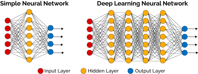
# Deep Learning
## Что это?
--

* Когда у нас есть исскуственная нейронная сеть

--

* Когда скрытых слоев в этой сети больше чем два

--


![](https://cdn-images-1.medium.com/max/1600/1*dnvGC-PORSoCo7VXT3PV_A.png)


.footnotes[[1] https://machinelearningmastery.com/what-is-deep-learning/]

---

## Как это математически
![](Deep_Learning_in_R_files/perceptron.png)

???

На самом деле это конечно самый простой юнит, самый базовый.

---
background-image: url(https://3qeqpr26caki16dnhd19sv6by6v-wpengine.netdna-ssl.com/wp-content/uploads/2016/08/Why-Deep-Learning-1024x742.png)

???

Image credit: [Andrew Ng](http://www.slideshare.net/ExtractConf)


---
class: inverse, center, middle, title-slide

# Frameworks
---
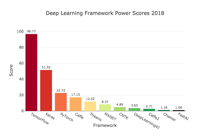
![](https://cdn-images-1.medium.com/max/1600/1*s_BwkYxpGv34vjOHi8tDzg.png)
.footnotes[
[1] https://towardsdatascience.com/deep-learning-framework-power-scores-2018-23607ddf297a
]
---
## Нас интересуют только те, что есть в R через API

--
* ###TensorFlow

--
* ###theano 

--
* ###Keras 

--
* ###CNTK 

--
* ###MXNet 

--
* ###ONNX 

---
## Есть еше несколько пакетов

* darch (removed from cran)

* deepnet

* deepr

* H2O (interface) ([Tutorial](https://htmlpreview.github.io/?https://github.com/ledell/sldm4-h2o/blob/master/sldm4-deeplearning-h2o.html))


???
Вода это по большей части МЛ фреймворк, с недавних пор, где появился модуль про глубокое обучение. Есть неплохой туториал для р пакета. Умеет в поиск гиперпараметров, кроссвалидацию и прочие нужные для МЛ штуки для сеток, очевидно это работает только для маленьких сетей)

Но они р специфичны, кроме воды, и соотвественно медленные, да и умеют довольно мало. Новые годные архитектуры сетей туда не имплементированы.

---
![](https://cdn-images-1.medium.com/max/1600/1*zmMOdVZ_j9vwMcpdD8Uceg.png)

https://www.tensorflow.org/

https://tensorflow.rstudio.com/

- Делает Google

- Самый популярный, имеет тучу туториалов и книг

- Имеет самый большой спрос у продакшн систем

- Имеет API во множестве языков

- Имеет статический граф вычислений, что бывает неудобно, зато оптимизированно

- Примерно с лета имеет фичу **eager execution**, который почти нивелирует это неудобство. Но почти не считается

- Доступен в R как самостоятельно, так и как бэкэнд Keras

---
![](https://cdn-images-1.medium.com/max/1600/1*dT-zhP2bmtxSuOja8gNGxA.png)

http://www.deeplearning.net/software/theano/

- Делался силами университета Монреаль с 2007

- Один из самый старых фреймворков, но почти почил в забытьи

- Придумали идею абстракции вычислительных графов (статических) для оптимизации и вычисления нейронных сетей

- В R доступен как бэкенд через Keras

---
![](https://cdn-images-1.medium.com/max/1600/1*tzgWkBhJPl5FFFe4uhn1AA.png)

https://cntk.ai/

- Делается силами Майкрософт

- Имеет половинчатые динамические вычислительные графы (на самом деле динамические тензоры скорее)

- Доступен как бэкенд Keras так и как самостоятельный бэкенд с биндингами в R через reticulate package, что значит нужно иметь python версию фреймворка

---
![](https://cdn-images-1.medium.com/max/1600/1*k9LIDsTb1K-Uejn7MCO7nA.png)

https://keras.io/

https://keras.rstudio.com/

https://tensorflow.rstudio.com/keras/

- Высокоуровневый фреймворк над другими такими бэкэндами как Theano, CNTK, Tensorflow, и еще некоторые на подходе
- Делается Франсуа Шолле, который написал книгу Deep Learning in R
- Очень простой код
- Один и тот же код рабоает на разных бэкендах, что теоретически может быть полезно (нет)
- Есть очень много блоков нейросетей из современных SOTA работ
- Нивелирует боль статических вычислительных графов
- Уже давно дефолтом поставляется вместе с TensorFlow как его часть, но можно использовать и отдельно


---
![](https://raw.githubusercontent.com/dmlc/web-data/master/mxnet/image/mxnet_logo_2.png)&lt;img src="https://raw.githubusercontent.com/dmlc/dmlc.github.io/master/img/logo-m/mxnetR.png" style=width:30% /&gt;

https://mxnet.apache.org/

https://github.com/apache/incubator-mxnet/tree/master/R-package

- Является проектом Apache

- Сочетает в себе динамические и статические графы

- Тоже имеет зоопарк предобученных моделей

- Как и TensorFlow поддерживается многими языками, что может быть очень полезно

- Довольно разумный и хороший фреймворк, непонятно, почему не пользуется популярностью


---
![](https://onnx.ai/onnx-r/articles/imgs/ONNX_logo_main.png)

https://onnx.ai/

https://onnx.ai/onnx-r/

- Предоставляет открытый формат представления вычислительных графов, чтобы можно было обмениваться запускать одни и теже, экспортированные в этот формат, модели с помощью разных фреймворков и своего рантайма

- Можно работать из R

- Изначально делался Microsoft вместе с Facebook

- Поддерживает кучу фреймворков нативно и конвертацию в ML и TF, Keras


---
class: inverse, middle, center

# Deep Learning with MXNet

---

## Установка 
В Windows и MacOS в R

```r
# Windows and MacOs 
cran &lt;- getOption("repos")
cran["dmlc"] &lt;- "https://apache-mxnet.s3-accelerate.dualstack.amazonaws.com/R/CRAN/GPU/cu92"
options(repos = cran)
install.packages("mxnet")
```

Linux bash

```bash
# On linux
git clone --recursive https://github.com/apache/incubator-mxnet.git mxnet
cd mxnet/docs/install
./install_mxnet_ubuntu_python.sh
./install_mxnet_ubuntu_r.sh

cd incubator-mxnet
make rpkg
```
---

## Загрузка и обработка данных

```r
df &lt;- read_csv("data.csv")
set.seed(100)
```


```r
#transform and split train on x and y
train_ind &lt;- sample(1:77, 60)
x_train &lt;- as.matrix(df[train_ind, 2:8])
y_train &lt;- unlist(df[train_ind, 9])
x_val &lt;- as.matrix(df[-train_ind, 2:8])
y_val &lt;- unlist(df[-train_ind, 9])
```

---
## Задания архитектуры сети


```r
require(mxnet)
# define graph
data &lt;- mx.symbol.Variable("data")

fc1 &lt;- mx.symbol.FullyConnected(data, num_hidden = 1)

linreg &lt;- mx.symbol.LinearRegressionOutput(fc1)

# define learing parameters
initializer &lt;- mx.init.normal(sd = 0.1)

optimizer &lt;- mx.opt.create("sgd", 
                           learning.rate = 1e-6,
                           momentum = 0.9)
# define logger

logger &lt;- mx.metric.logger()
epoch.end.callback &lt;- mx.callback.log.train.metric(
  period = 4, # число батчей, после которого оценивается метрика
  logger = logger)

# num of epoch
n_epoch &lt;- 20
```

---
## Построим граф модели

```r
# plot our model
graph.viz(linreg)
```
&lt;img src="Deep_Learning_in_R_files/graph.png" style="width:50%" &gt;

---
## Обучим

```r
model &lt;- mx.model.FeedForward.create(
  symbol = linreg, # our model
  X = x_train, # our data
  y = y_train, # our label
  ctx = mx.cpu(), # engine
  num.round = n_epoch, 
  initializer = initializer, # inizialize weigths
  optimizer = optimizer, # sgd optimizer
  eval.data = list(data = x_val, label = y_val), # evaluation on evey epoch
  eval.metric = mx.metric.rmse, # metric
  array.batch.size = 15, 
  epoch.end.callback = epoch.end.callback) # logger
```

```
## Warning in mx.model.select.layout.train(X, y): Auto detect layout of input matrix, use rowmajor..
```

```
## Start training with 1 devices
```

```
## [1] Train-rmse=7.85010987520218
```

```
## [1] Validation-rmse=7.99821019172668
```

```
## [2] Train-rmse=9.21365368366241
```

```
## [2] Validation-rmse=4.74030923843384
```

```
## [3] Train-rmse=4.16309010982513
```

```
## [3] Validation-rmse=7.18643116950989
```

```
## [4] Train-rmse=5.20915931463242
```

```
## [4] Validation-rmse=3.87698078155518
```

```
## [5] Train-rmse=4.94802039861679
```

```
## [5] Validation-rmse=3.80227029323578
```

```
## [6] Train-rmse=2.69853216409683
```

```
## [6] Validation-rmse=3.90478467941284
```

```
## [7] Train-rmse=3.52689051628113
```

```
## [7] Validation-rmse=2.31562197208405
```

```
## [8] Train-rmse=2.99551945924759
```

```
## [8] Validation-rmse=2.93496096134186
```

```
## [9] Train-rmse=2.22769635915756
```

```
## [9] Validation-rmse=2.37067186832428
```

```
## [10] Train-rmse=2.5699103474617
```

```
## [10] Validation-rmse=1.86853647232056
```

```
## [11] Train-rmse=2.24543181061745
```

```
## [11] Validation-rmse=2.3385466337204
```

```
## [12] Train-rmse=2.03947871923447
```

```
## [12] Validation-rmse=1.82985359430313
```

```
## [13] Train-rmse=2.111790984869
```

```
## [13] Validation-rmse=1.74209445714951
```

```
## [14] Train-rmse=1.98190069198608
```

```
## [14] Validation-rmse=1.98799872398376
```

```
## [15] Train-rmse=1.9320664703846
```

```
## [15] Validation-rmse=1.68956047296524
```

```
## [16] Train-rmse=1.91881200671196
```

```
## [16] Validation-rmse=1.68268179893494
```

```
## [17] Train-rmse=1.87585905194283
```

```
## [17] Validation-rmse=1.79575181007385
```

```
## [18] Train-rmse=1.85955160856247
```

```
## [18] Validation-rmse=1.64644628763199
```

```
## [19] Train-rmse=1.83187100291252
```

```
## [19] Validation-rmse=1.63903748989105
```

```
## [20] Train-rmse=1.81522011756897
```

```
## [20] Validation-rmse=1.68724113702774
```

---
## Построим кривую обучения

```r
rmse_log &lt;- data.frame(RMSE = c(logger$train, logger$eval),dataset = c(rep("train", length(logger$train)),                        rep("val", length(logger$eval))),epoch = 1:n_epoch)
library(ggplot2)
ggplot(rmse_log, aes(epoch, RMSE, group = dataset, colour = dataset)) +  geom_point() +  geom_line()
```

![](Deep_Learning_in_R_files/figure-html/unnamed-chunk-7-1.svg)&lt;!-- --&gt;

---
class: inverse, center, middle
# Deep Learning with Keras

---
## Установка

```r
install.packages("keras")
keras::install_keras(tensorflow = 'gpu')
```
### Загрузка нужных нам пакетов

```r
require(keras)     # Neural Networks
require(tidyverse) # Data cleaning / Visualization
require(knitr)     # Table printing
require(rmarkdown) # Misc. output utilities 
require(ggridges)  # Visualization
```

---
## Загрузка данных

```r
activityLabels &lt;- read.table("Deep_Learning_in_R_files/HAPT Data Set/activity_labels.txt", 
                             col.names = c("number", "label")) 
activityLabels %&gt;% kable(align = c("c", "l"))
```


 number   label              
--------  -------------------
   1      WALKING            
   2      WALKING_UPSTAIRS   
   3      WALKING_DOWNSTAIRS 
   4      SITTING            
   5      STANDING           
   6      LAYING             
   7      STAND_TO_SIT       
   8      SIT_TO_STAND       
   9      SIT_TO_LIE         
   10     LIE_TO_SIT         
   11     STAND_TO_LIE       
   12     LIE_TO_STAND       

---

```r
labels &lt;- read.table("Deep_Learning_in_R_files/HAPT Data Set/RawData/labels.txt",
                     col.names = c("experiment", "userId", "activity", "startPos", "endPos"))
dataFiles &lt;- list.files("Deep_Learning_in_R_files/HAPT Data Set/RawData")
labels %&gt;% 
  head(50) %&gt;% 
  paged_table()
```

&lt;div data-pagedtable="false"&gt;
  &lt;script data-pagedtable-source type="application/json"&gt;
{"columns":[{"label":[""],"name":["_rn_"],"type":[""],"align":["left"]},{"label":["experiment"],"name":[1],"type":["int"],"align":["right"]},{"label":["userId"],"name":[2],"type":["int"],"align":["right"]},{"label":["activity"],"name":[3],"type":["int"],"align":["right"]},{"label":["startPos"],"name":[4],"type":["int"],"align":["right"]},{"label":["endPos"],"name":[5],"type":["int"],"align":["right"]}],"data":[{"1":"1","2":"1","3":"5","4":"250","5":"1232","_rn_":"1"},{"1":"1","2":"1","3":"7","4":"1233","5":"1392","_rn_":"2"},{"1":"1","2":"1","3":"4","4":"1393","5":"2194","_rn_":"3"},{"1":"1","2":"1","3":"8","4":"2195","5":"2359","_rn_":"4"},{"1":"1","2":"1","3":"5","4":"2360","5":"3374","_rn_":"5"},{"1":"1","2":"1","3":"11","4":"3375","5":"3662","_rn_":"6"},{"1":"1","2":"1","3":"6","4":"3663","5":"4538","_rn_":"7"},{"1":"1","2":"1","3":"10","4":"4539","5":"4735","_rn_":"8"},{"1":"1","2":"1","3":"4","4":"4736","5":"5667","_rn_":"9"},{"1":"1","2":"1","3":"9","4":"5668","5":"5859","_rn_":"10"},{"1":"1","2":"1","3":"6","4":"5860","5":"6786","_rn_":"11"},{"1":"1","2":"1","3":"12","4":"6787","5":"6977","_rn_":"12"},{"1":"1","2":"1","3":"1","4":"7496","5":"8078","_rn_":"13"},{"1":"1","2":"1","3":"1","4":"8356","5":"9250","_rn_":"14"},{"1":"1","2":"1","3":"1","4":"9657","5":"10567","_rn_":"15"},{"1":"1","2":"1","3":"1","4":"10750","5":"11714","_rn_":"16"},{"1":"1","2":"1","3":"3","4":"13191","5":"13846","_rn_":"17"},{"1":"1","2":"1","3":"2","4":"14069","5":"14699","_rn_":"18"},{"1":"1","2":"1","3":"3","4":"14869","5":"15492","_rn_":"19"},{"1":"1","2":"1","3":"2","4":"15712","5":"16377","_rn_":"20"},{"1":"1","2":"1","3":"3","4":"16530","5":"17153","_rn_":"21"},{"1":"1","2":"1","3":"2","4":"17298","5":"17970","_rn_":"22"},{"1":"2","2":"1","3":"5","4":"251","5":"1226","_rn_":"23"},{"1":"2","2":"1","3":"7","4":"1227","5":"1432","_rn_":"24"},{"1":"2","2":"1","3":"4","4":"1433","5":"2221","_rn_":"25"},{"1":"2","2":"1","3":"8","4":"2222","5":"2377","_rn_":"26"},{"1":"2","2":"1","3":"5","4":"2378","5":"3304","_rn_":"27"},{"1":"2","2":"1","3":"11","4":"3305","5":"3572","_rn_":"28"},{"1":"2","2":"1","3":"6","4":"3573","5":"4435","_rn_":"29"},{"1":"2","2":"1","3":"10","4":"4436","5":"4619","_rn_":"30"},{"1":"2","2":"1","3":"4","4":"4620","5":"5452","_rn_":"31"},{"1":"2","2":"1","3":"9","4":"5453","5":"5689","_rn_":"32"},{"1":"2","2":"1","3":"6","4":"5690","5":"6467","_rn_":"33"},{"1":"2","2":"1","3":"12","4":"6468","5":"6709","_rn_":"34"},{"1":"2","2":"1","3":"1","4":"7624","5":"8252","_rn_":"35"},{"1":"2","2":"1","3":"1","4":"8618","5":"9576","_rn_":"36"},{"1":"2","2":"1","3":"1","4":"9991","5":"10927","_rn_":"37"},{"1":"2","2":"1","3":"1","4":"11311","5":"12282","_rn_":"38"},{"1":"2","2":"1","3":"3","4":"13129","5":"13379","_rn_":"39"},{"1":"2","2":"1","3":"3","4":"13495","5":"13927","_rn_":"40"},{"1":"2","2":"1","3":"2","4":"14128","5":"14783","_rn_":"41"},{"1":"2","2":"1","3":"3","4":"15037","5":"15684","_rn_":"42"},{"1":"2","2":"1","3":"2","4":"15920","5":"16598","_rn_":"43"},{"1":"2","2":"1","3":"3","4":"16847","5":"17471","_rn_":"44"},{"1":"2","2":"1","3":"2","4":"17725","5":"18425","_rn_":"45"},{"1":"3","2":"2","3":"5","4":"298","5":"1398","_rn_":"46"},{"1":"3","2":"2","3":"7","4":"1399","5":"1555","_rn_":"47"},{"1":"3","2":"2","3":"4","4":"1686","5":"2627","_rn_":"48"},{"1":"3","2":"2","3":"8","4":"2628","5":"2769","_rn_":"49"},{"1":"3","2":"2","3":"5","4":"2770","5":"3904","_rn_":"50"}],"options":{"columns":{"min":{},"max":[10]},"rows":{"min":[10],"max":[10]},"pages":{}}}
  &lt;/script&gt;
&lt;/div&gt;

---

```r
fileInfo &lt;- data_frame(
  filePath = dataFiles
) %&gt;%
  filter(filePath != "labels.txt") %&gt;% 
  separate(filePath, sep = '_', 
           into = c("type", "experiment", "userId"), 
           remove = FALSE) %&gt;% 
  mutate(
    experiment = str_remove(experiment, "exp"),
    userId = str_remove_all(userId, "user|\\.txt")
  ) %&gt;% 
  spread(type, filePath)

fileInfo %&gt;% head() %&gt;% kable()
```


experiment   userId   acc                    gyro                  
-----------  -------  ---------------------  ----------------------
01           01       acc_exp01_user01.txt   gyro_exp01_user01.txt 
02           01       acc_exp02_user01.txt   gyro_exp02_user01.txt 
03           02       acc_exp03_user02.txt   gyro_exp03_user02.txt 
04           02       acc_exp04_user02.txt   gyro_exp04_user02.txt 
05           03       acc_exp05_user03.txt   gyro_exp05_user03.txt 
06           03       acc_exp06_user03.txt   gyro_exp06_user03.txt 
---
# remark.js

Some differences between using remark.js (left) and using **xaringan** (right):

.pull-left[
1. Start with a boilerplate HTML file;

1. Plain Markdown;

1. Write JavaScript to autoplay slides;

1. Manually configure MathJax;

1. Highlight code with `*`;

1. Edit Markdown source and refresh browser to see updated slides;
]

.pull-right[
1. Start with an R Markdown document;

1. R Markdown (can embed R/other code chunks);

1. Provide an option `autoplay`;

1. MathJax just works;&lt;sup&gt;*&lt;/sup&gt;

1. Highlight code with `{{}}`;

1. The RStudio addin "Infinite Moon Reader" automatically refreshes slides on changes;
]

.footnote[[*] Not really. See next page.]

---

# Math Expressions

You can write LaTeX math expressions inside a pair of dollar signs, e.g. &amp;#36;\alpha+\beta$ renders `\(\alpha+\beta\)`. You can use the display style with double dollar signs:

```
$$\bar{X}=\frac{1}{n}\sum_{i=1}^nX_i$$
```

`$$\bar{X}=\frac{1}{n}\sum_{i=1}^nX_i$$`

Limitations:

1. The source code of a LaTeX math expression must be in one line, unless it is inside a pair of double dollar signs, in which case the starting `$$` must appear in the very beginning of a line, followed immediately by a non-space character, and the ending `$$` must be at the end of a line, led by a non-space character;

1. There should not be spaces after the opening `$` or before the closing `$`.

1. Math does not work on the title slide (see [#61](https://github.com/yihui/xaringan/issues/61) for a workaround).

---

# R Code


```r
# a boring regression
fit = lm(dist ~ 1 + speed, data = cars)
coef(summary(fit))
```

```
#               Estimate Std. Error   t value     Pr(&gt;|t|)
# (Intercept) -17.579095  6.7584402 -2.601058 1.231882e-02
# speed         3.932409  0.4155128  9.463990 1.489836e-12
```

```r
dojutsu = c('地爆天星', '天照', '加具土命', '神威', '須佐能乎', '無限月読')
grep('天', dojutsu, value = TRUE)
```

```
# character(0)
```

---

# R Plots


```r
par(mar = c(4, 4, 1, .1))
plot(cars, pch = 19, col = 'darkgray', las = 1)
abline(fit, lwd = 2)
```

![](Deep_Learning_in_R_files/figure-html/cars-1.svg)&lt;!-- --&gt;

---

# Tables

If you want to generate a table, make sure it is in the HTML format (instead of Markdown or other formats), e.g.,


```r
knitr::kable(head(iris), format = 'html')
```

&lt;table&gt;
 &lt;thead&gt;
  &lt;tr&gt;
   &lt;th style="text-align:right;"&gt; Sepal.Length &lt;/th&gt;
   &lt;th style="text-align:right;"&gt; Sepal.Width &lt;/th&gt;
   &lt;th style="text-align:right;"&gt; Petal.Length &lt;/th&gt;
   &lt;th style="text-align:right;"&gt; Petal.Width &lt;/th&gt;
   &lt;th style="text-align:left;"&gt; Species &lt;/th&gt;
  &lt;/tr&gt;
 &lt;/thead&gt;
&lt;tbody&gt;
  &lt;tr&gt;
   &lt;td style="text-align:right;"&gt; 5.1 &lt;/td&gt;
   &lt;td style="text-align:right;"&gt; 3.5 &lt;/td&gt;
   &lt;td style="text-align:right;"&gt; 1.4 &lt;/td&gt;
   &lt;td style="text-align:right;"&gt; 0.2 &lt;/td&gt;
   &lt;td style="text-align:left;"&gt; setosa &lt;/td&gt;
  &lt;/tr&gt;
  &lt;tr&gt;
   &lt;td style="text-align:right;"&gt; 4.9 &lt;/td&gt;
   &lt;td style="text-align:right;"&gt; 3.0 &lt;/td&gt;
   &lt;td style="text-align:right;"&gt; 1.4 &lt;/td&gt;
   &lt;td style="text-align:right;"&gt; 0.2 &lt;/td&gt;
   &lt;td style="text-align:left;"&gt; setosa &lt;/td&gt;
  &lt;/tr&gt;
  &lt;tr&gt;
   &lt;td style="text-align:right;"&gt; 4.7 &lt;/td&gt;
   &lt;td style="text-align:right;"&gt; 3.2 &lt;/td&gt;
   &lt;td style="text-align:right;"&gt; 1.3 &lt;/td&gt;
   &lt;td style="text-align:right;"&gt; 0.2 &lt;/td&gt;
   &lt;td style="text-align:left;"&gt; setosa &lt;/td&gt;
  &lt;/tr&gt;
  &lt;tr&gt;
   &lt;td style="text-align:right;"&gt; 4.6 &lt;/td&gt;
   &lt;td style="text-align:right;"&gt; 3.1 &lt;/td&gt;
   &lt;td style="text-align:right;"&gt; 1.5 &lt;/td&gt;
   &lt;td style="text-align:right;"&gt; 0.2 &lt;/td&gt;
   &lt;td style="text-align:left;"&gt; setosa &lt;/td&gt;
  &lt;/tr&gt;
  &lt;tr&gt;
   &lt;td style="text-align:right;"&gt; 5.0 &lt;/td&gt;
   &lt;td style="text-align:right;"&gt; 3.6 &lt;/td&gt;
   &lt;td style="text-align:right;"&gt; 1.4 &lt;/td&gt;
   &lt;td style="text-align:right;"&gt; 0.2 &lt;/td&gt;
   &lt;td style="text-align:left;"&gt; setosa &lt;/td&gt;
  &lt;/tr&gt;
  &lt;tr&gt;
   &lt;td style="text-align:right;"&gt; 5.4 &lt;/td&gt;
   &lt;td style="text-align:right;"&gt; 3.9 &lt;/td&gt;
   &lt;td style="text-align:right;"&gt; 1.7 &lt;/td&gt;
   &lt;td style="text-align:right;"&gt; 0.4 &lt;/td&gt;
   &lt;td style="text-align:left;"&gt; setosa &lt;/td&gt;
  &lt;/tr&gt;
&lt;/tbody&gt;
&lt;/table&gt;

---

# HTML Widgets

I have not thoroughly tested HTML widgets against **xaringan**. Some may work well, and some may not. It is a little tricky.

Similarly, the Shiny mode (`runtime: shiny`) does not work. I might get these issues fixed in the future, but these are not of high priority to me. I never turn my presentation into a Shiny app. When I need to demonstrate more complicated examples, I just launch them separately. It is convenient to share slides with other people when they are plain HTML/JS applications.

See the next page for two HTML widgets.

---


```r
library(leaflet)
leaflet() %&gt;% addTiles() %&gt;% setView(-93.65, 42.0285, zoom = 17)
```

<div id="htmlwidget-b7ecac2f591f1b4cd6fe" style="width:100%;height:432px;" class="leaflet html-widget"></div>
<script type="application/json" data-for="htmlwidget-b7ecac2f591f1b4cd6fe">{"x":{"options":{"crs":{"crsClass":"L.CRS.EPSG3857","code":null,"proj4def":null,"projectedBounds":null,"options":{}}},"calls":[{"method":"addTiles","args":["//{s}.tile.openstreetmap.org/{z}/{x}/{y}.png",null,null,{"minZoom":0,"maxZoom":18,"tileSize":256,"subdomains":"abc","errorTileUrl":"","tms":false,"noWrap":false,"zoomOffset":0,"zoomReverse":false,"opacity":1,"zIndex":1,"detectRetina":false,"attribution":"&copy; <a href=\"http://openstreetmap.org\">OpenStreetMap<\/a> contributors, <a href=\"http://creativecommons.org/licenses/by-sa/2.0/\">CC-BY-SA<\/a>"}]}],"setView":[[42.0285,-93.65],17,[]]},"evals":[],"jsHooks":[]}</script>

---


```r
DT::datatable(
  head(iris, 10),
  fillContainer = FALSE, options = list(pageLength = 8)
)
```

<div id="htmlwidget-6f33f6a94c1e991ec95e" style="width:100%;height:auto;" class="datatables html-widget"></div>
<script type="application/json" data-for="htmlwidget-6f33f6a94c1e991ec95e">{"x":{"filter":"none","fillContainer":false,"data":[["1","2","3","4","5","6","7","8","9","10"],[5.1,4.9,4.7,4.6,5,5.4,4.6,5,4.4,4.9],[3.5,3,3.2,3.1,3.6,3.9,3.4,3.4,2.9,3.1],[1.4,1.4,1.3,1.5,1.4,1.7,1.4,1.5,1.4,1.5],[0.2,0.2,0.2,0.2,0.2,0.4,0.3,0.2,0.2,0.1],["setosa","setosa","setosa","setosa","setosa","setosa","setosa","setosa","setosa","setosa"]],"container":"<table class=\"display\">\n  <thead>\n    <tr>\n      <th> <\/th>\n      <th>Sepal.Length<\/th>\n      <th>Sepal.Width<\/th>\n      <th>Petal.Length<\/th>\n      <th>Petal.Width<\/th>\n      <th>Species<\/th>\n    <\/tr>\n  <\/thead>\n<\/table>","options":{"pageLength":8,"columnDefs":[{"className":"dt-right","targets":[1,2,3,4]},{"orderable":false,"targets":0}],"order":[],"autoWidth":false,"orderClasses":false,"lengthMenu":[8,10,25,50,100]}},"evals":[],"jsHooks":[]}</script>

---

# Some Tips

- When you use the "Infinite Moon Reader" addin in RStudio, your R session will be blocked by default. You can click the red button on the right of the console to stop serving the slides, or use the _daemonized_ mode so that it does not block your R session. To do the latter, you can set the option

    ```r
    options(servr.daemon = TRUE)
    ```
    
    in your current R session, or in `~/.Rprofile` so that it is applied to all future R sessions. I do the latter by myself.
    
    To know more about the web server, see the [**servr**](https://github.com/yihui/servr) package.

--

- Do not forget to try the `yolo` option of `xaringan::moon_reader`.

    ```yaml
    output:
      xaringan::moon_reader:
        yolo: true
    ```

---

# Some Tips

- Slides can be automatically played if you set the `autoplay` option under `nature`, e.g. go to the next slide every 30 seconds in a lightning talk:

    ```yaml
    output:
      xaringan::moon_reader:
        nature:
          autoplay: 30000
    ```

--

- A countdown timer can be added to every page of the slides using the `countdown` option under `nature`, e.g. if you want to spend one minute on every page when you give the talk, you can set:

    ```yaml
    output:
      xaringan::moon_reader:
        nature:
          countdown: 60000
    ```

    Then you will see a timer counting down from `01:00`, to `00:59`, `00:58`, ... When the time is out, the timer will continue but the time turns red.

---

# Some Tips

- There are several ways to build incremental slides. See [this presentation](https://slides.yihui.name/xaringan/incremental.html) for examples.

- The option `highlightLines: true` of `nature` will highlight code lines that start with `*`, or are wrapped in `{{ }}`, or have trailing comments `#&lt;&lt;`;

    ```yaml
    output:
      xaringan::moon_reader:
        nature:
          highlightLines: true
    ```

    See examples on the next page.

---

# Some Tips


.pull-left[
An example using a leading `*`:

    ```r
    if (TRUE) {
    ** message("Very important!")
    }
    ```
Output:
```r
if (TRUE) {
* message("Very important!")
}
```

This is invalid R code, so it is a plain fenced code block that is not executed.
]

.pull-right[
An example using `{{}}`:

    ```{r tidy=FALSE}
    if (TRUE) {
    *{{ message("Very important!") }}
    }
    ```
Output:

```r
if (TRUE) {
* message("Very important!") 
}
```

```
## Very important!
```

It is valid R code so you can run it. Note that `{{}}` can wrap an R expression of multiple lines.
]

---

# Some Tips

An example of using the trailing comment `#&lt;&lt;` to highlight lines:

````markdown
```{r tidy=FALSE}
library(ggplot2)
ggplot(mtcars) + 
  aes(mpg, disp) + 
  geom_point() +   #&lt;&lt;
  geom_smooth()    #&lt;&lt;
```
````

Output:


```r
library(ggplot2)
ggplot(mtcars) + 
  aes(mpg, disp) + 
* geom_point() +
* geom_smooth()
```

---

# Some Tips

- To make slides work offline, you need to download a copy of remark.js in advance, because **xaringan** uses the online version by default (see the help page `?xaringan::moon_reader`).

- You can use `xaringan::summon_remark()` to download the latest or a specified version of remark.js. By default, it is downloaded to `libs/remark-latest.min.js`.

- Then change the `chakra` option in YAML to point to this file, e.g.

    ```yaml
    output:
      xaringan::moon_reader:
        chakra: libs/remark-latest.min.js
    ```

- If you used Google fonts in slides (the default theme uses _Yanone Kaffeesatz_, _Droid Serif_, and _Source Code Pro_), they won't work offline unless you download or install them locally. The Heroku app [google-webfonts-helper](https://google-webfonts-helper.herokuapp.com/fonts) can help you download fonts and generate the necessary CSS.

---

# Macros

- remark.js [allows users to define custom macros](https://github.com/yihui/xaringan/issues/80) (JS functions) that can be applied to Markdown text using the syntax `![:macroName arg1, arg2, ...]` or `![:macroName arg1, arg2, ...](this)`. For example, before remark.js initializes the slides, you can define a macro named `scale`:

    ```js
    remark.macros.scale = function (percentage) {
      var url = this;
      return '&lt;img src="' + url + '" style="width: ' + percentage + '" /&gt;';
    };
    ```

    Then the Markdown text

    ```markdown
    ![:scale 50%](image.jpg)
    ```

    will be translated to
    
    ```html
    &lt;img src="image.jpg" style="width: 50%" /&gt;
    ```

---

# Macros (continued)

- To insert macros in **xaringan** slides, you can use the option `beforeInit` under the option `nature`, e.g.,

    ```yaml
    output:
      xaringan::moon_reader:
        nature:
          beforeInit: "macros.js"
    ```

    You save your remark.js macros in the file `macros.js`.

- The `beforeInit` option can be used to insert arbitrary JS code before `remark.create()`. Inserting macros is just one of its possible applications.

---

# CSS

Among all options in `xaringan::moon_reader`, the most challenging but perhaps also the most rewarding one is `css`, because it allows you to customize the appearance of your slides using any CSS rules or hacks you know.

You can see the default CSS file [here](https://github.com/yihui/xaringan/blob/master/inst/rmarkdown/templates/xaringan/resources/default.css). You can completely replace it with your own CSS files, or define new rules to override the default. See the help page `?xaringan::moon_reader` for more information.

---

# CSS

For example, suppose you want to change the font for code from the default "Source Code Pro" to "Ubuntu Mono". You can create a CSS file named, say, `ubuntu-mono.css`:

```css
@import url(https://fonts.googleapis.com/css?family=Ubuntu+Mono:400,700,400italic);

.remark-code, .remark-inline-code { font-family: 'Ubuntu Mono'; }
```

Then set the `css` option in the YAML metadata:

```yaml
output:
  xaringan::moon_reader:
    css: ["default", "ubuntu-mono.css"]
```

Here I assume `ubuntu-mono.css` is under the same directory as your Rmd.

See [yihui/xaringan#83](https://github.com/yihui/xaringan/issues/83) for an example of using the [Fira Code](https://github.com/tonsky/FiraCode) font, which supports ligatures in program code.

---

# Themes

Don't want to learn CSS? Okay, you can use some user-contributed themes. A theme typically consists of two CSS files `foo.css` and `foo-fonts.css`, where `foo` is the theme name. Below are some existing themes:


```r
names(xaringan:::list_css())
```

```
##  [1] "chocolate-fonts"  "chocolate"        "default-fonts"   
##  [4] "default"          "duke-blue"        "hygge-duke"      
##  [7] "hygge"            "kunoichi"         "lucy-fonts"      
## [10] "lucy"             "metropolis-fonts" "metropolis"      
## [13] "middlebury-fonts" "middlebury"       "ninjutsu"        
## [16] "rladies-fonts"    "rladies"          "robot-fonts"     
## [19] "robot"            "rutgers-fonts"    "rutgers"         
## [22] "shinobi"          "tamu-fonts"       "tamu"            
## [25] "uo-fonts"         "uo"
```

To use a theme, you can specify the `css` option as an array of CSS filenames (without the `.css` extensions), e.g.,

```yaml
output:
  xaringan::moon_reader:
    css: [default, metropolis, metropolis-fonts]
```

If you want to contribute a theme to **xaringan**, please read [this blog post](https://yihui.name/en/2017/10/xaringan-themes).

---
class: inverse, middle, center
background-image: url(https://upload.wikimedia.org/wikipedia/commons/3/39/Naruto_Shiki_Fujin.svg)
background-size: contain

# Naruto

---
background-image: url(https://upload.wikimedia.org/wikipedia/commons/b/be/Sharingan_triple.svg)
background-size: 100px
background-position: 90% 8%

# Sharingan

The R package name **xaringan** was derived&lt;sup&gt;1&lt;/sup&gt; from **Sharingan**, a dōjutsu in the Japanese anime _Naruto_ with two abilities:

- the "Eye of Insight"

- the "Eye of Hypnotism"

I think a presentation is basically a way to communicate insights to the audience, and a great presentation may even "hypnotize" the audience.&lt;sup&gt;2,3&lt;/sup&gt;

.footnote[
[1] In Chinese, the pronounciation of _X_ is _Sh_ /ʃ/ (as in _shrimp_). Now you should have a better idea of how to pronounce my last name _Xie_.

[2] By comparison, bad presentations only put the audience to sleep.

[3] Personally I find that setting background images for slides is a killer feature of remark.js. It is an effective way to bring visual impact into your presentations.
]

---

# Naruto terminology

The **xaringan** package borrowed a few terms from Naruto, such as

- [Sharingan](http://naruto.wikia.com/wiki/Sharingan) (写輪眼; the package name)

- The [moon reader](http://naruto.wikia.com/wiki/Moon_Reader) (月読; an attractive R Markdown output format)

- [Chakra](http://naruto.wikia.com/wiki/Chakra) (查克拉; the path to the remark.js library, which is the power to drive the presentation)

- [Nature transformation](http://naruto.wikia.com/wiki/Nature_Transformation) (性質変化; transform the chakra by setting different options)

- The [infinite moon reader](http://naruto.wikia.com/wiki/Infinite_Tsukuyomi) (無限月読; start a local web server to continuously serve your slides)

- The [summoning technique](http://naruto.wikia.com/wiki/Summoning_Technique) (download remark.js from the web)

You can click the links to know more about them if you want. The jutsu "Moon Reader" may seem a little evil, but that does not mean your slides are evil.

---

class: center

# Hand seals (印)

Press `h` or `?` to see the possible ninjutsu you can use in remark.js.

![](https://upload.wikimedia.org/wikipedia/commons/7/7e/Mudra-Naruto-KageBunshin.svg)

---

class: center, middle

# Thanks!

Slides created via the R package [**xaringan**](https://github.com/yihui/xaringan).

The chakra comes from [remark.js](https://remarkjs.com), [**knitr**](http://yihui.name/knitr), and [R Markdown](https://rmarkdown.rstudio.com).
    </textarea>
<script src="https://remarkjs.com/downloads/remark-latest.min.js"></script>
<script>var slideshow = remark.create({
"highlightStyle": "github",
"highlightLines": true,
"countIncrementalSlides": false
});
if (window.HTMLWidgets) slideshow.on('afterShowSlide', function (slide) {
  window.dispatchEvent(new Event('resize'));
});
(function() {
  var d = document, s = d.createElement("style"), r = d.querySelector(".remark-slide-scaler");
  if (!r) return;
  s.type = "text/css"; s.innerHTML = "@page {size: " + r.style.width + " " + r.style.height +"; }";
  d.head.appendChild(s);
})();</script>

<script>
(function() {
  var i, text, code, codes = document.getElementsByTagName('code');
  for (i = 0; i < codes.length;) {
    code = codes[i];
    if (code.parentNode.tagName !== 'PRE' && code.childElementCount === 0) {
      text = code.textContent;
      if (/^\\\((.|\s)+\\\)$/.test(text) || /^\\\[(.|\s)+\\\]$/.test(text) ||
          /^\$\$(.|\s)+\$\$$/.test(text) ||
          /^\\begin\{([^}]+)\}(.|\s)+\\end\{[^}]+\}$/.test(text)) {
        code.outerHTML = code.innerHTML;  // remove <code></code>
        continue;
      }
    }
    i++;
  }
})();
</script>
<!-- dynamically load mathjax for compatibility with self-contained -->
<script>
(function () {
  var script = document.createElement('script');
  script.type = 'text/javascript';
  script.src  = 'https://mathjax.rstudio.com/latest/MathJax.js?config=TeX-MML-AM_CHTML';
  if (location.protocol !== 'file:' && /^https?:/.test(script.src))
    script.src  = script.src.replace(/^https?:/, '');
  document.getElementsByTagName('head')[0].appendChild(script);
})();
</script>
  </body>
</html>